Snow depths with PDAL

For the past several years we've been using terrestrial LiDAR to monitor snow-covered mountainsides for avalanche stability and mitigation. We've even gotten some local press for our efforts. We just completed processing for our data from the Seven Sisters at Loveland Pass, CO, where we've been working with the Colorado Department of Transportation (CDOT) to assess the effectivity of their installed GasEx systems. I used PDAL to calculate and visualize the height of snow (HS) for these data, and the process was non-trivial enough to be worth a blog post.

Source data

The data were georeferenced using Riegl's proprietary RiSCAN Pro and exported to the laz format. Our workflow uses UTM coordiantes inside RiSCAN Pro, which doesn't play nicely with Riegl's GeoSysManager, so the georeferenced laz files from RiSCAN Pro don't have correct spatial reference information in the las header. Additionaly, as seen below, there's a lot of in-air noise (usually due to blowing snow) and a lot of high-density points near that scanner that we aren't really interested in.

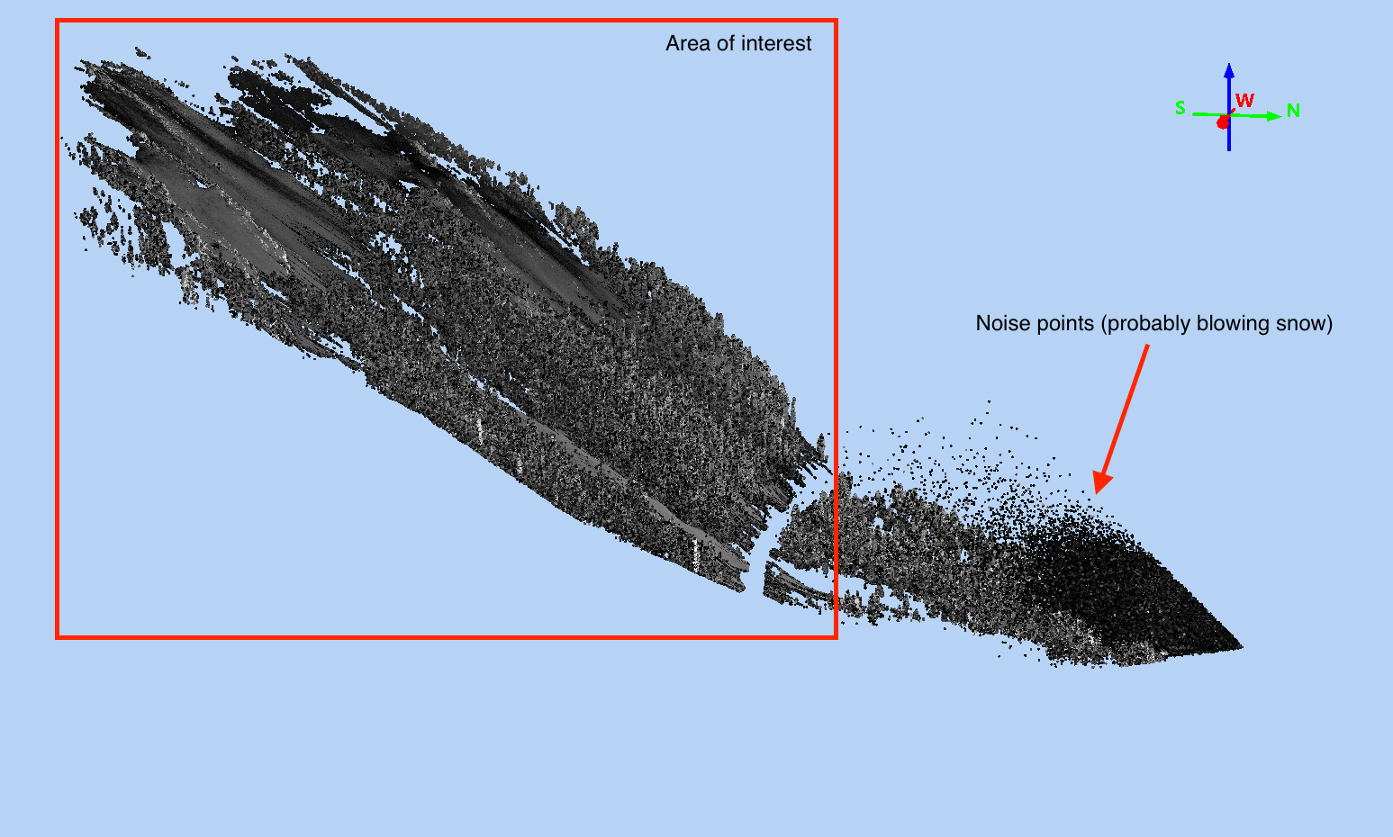
We're also interested in removing all the trees in the scan, as we only really want a bare earth surface and the snow surface for our HS measurements.

Generating reference surfaces

The first step is to post-process the point clouds, as delivered from Riegl, using the following pipeline:

{
    "pipeline": [
        {
            "type": "readers.las",
            "spatialreference": "EPSG:6342+5703"
        },
        {
            "type": "filters.crop",
            "polygon": "POLYGON((424285.054199 4392521.066437,424264.463623 4392406.715332,424205.290527 4392190.98584,424201.560547 4392140.775757,423641.87146 4391921.607422,423426.168762 4391845.724854,423401.804596 4391842.146729,423041.956669 4392012.294861,422662.966858 4392335.28717,422759.23587 4392382.745789,422961.488438 4392474.017517,423273.389465 4392601.933075,423419.496582 4392539.133209,423538.245728 4392509.673706,423915.109497 4392511.763214,424070.769165 4392542.10498,424201.549438 4392565.36734,424248.287964 4392556.360779,424280.257935 4392531.412476,424285.054199 4392521.066437))"
        },
        {
            "type": "filters.outlier"
        },
        {
            "type": "filters.smrf",
            "ignore": "Classification[7:7]"
        },
        {
            "type": "writers.las"
        }
    ]
}

Step-by-step, this pipeline:

1. Reads in the las data and tags it as UTM 13N / NAD83(2011)¹, with the NAVD88 vertical datum.
2. Crops the data to a pre-defined area of interest.
3. Uses the outlier filter to add the classifation value "7" (Low point/Noise) to all noise points.
4. Classifies all ground points using PDAL's smrf filter, ignoring noise points. Note that for snow-on scans, we're hoping that both bare ground and snow surfaces get classified as ground.
5. Writes out the data to a las file.

You'll notice that neither the readers.las stage or the writers.las stage have filenames specified; this is because we use this pipeline via the following makefile rule. The same concept applies for all future pipelines, as well:

build/full-resolution/%: laz/from-riscan/% pipelines/from-riscan.json
 @mkdir -p $(dir $@)
 pdal pipeline pipelines/from-riscan.json \
  --readers.las.filename="$<" \
  --writers.las.filename="$@"

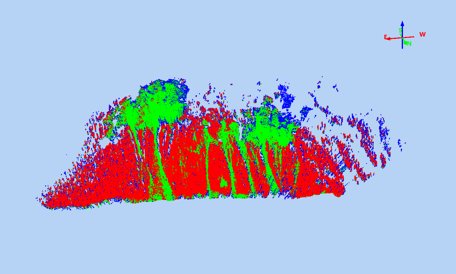
This lets us quickly create full-resolution processed laz files in parallel using a simple make command e.g. make -j 6 all, Our full resolution, classified point cloud might look like this, colorized by classification (green: ground/snow, blue: noise, red: non-ground/snow):

With the full resolution, classified points, we then can create bare-earth (or bare-snow) surfaces for each scan. The bare-earth surface from our snow-off scan will be the reference surface for all snow depth (HS) calculations, and the bare-snow surfaces from snow-on scans will be used for change in snow depth (dHS) calculations, which are useful for analysing the distribution of snow depth after a storm or identifying the snow removed/deposited by an avalanche. To create the bare-earth/bare-snow surfaces, we use the following pipeline:

{
    "pipeline": [
        {
            "type": "readers.las"
        },
        {
            "type": "filters.range",
            "limits": "Classification[2:2]"
        },
        {
            "type": "writers.gdal",
            "resolution": 0.5,
            "output_type": "min",
            "window_size": 2
        }
    ]
}

The "2" classifications were added by the filters.smrf, and we choose a 0.5m resolution for our raster.

Calculating snow depths

Once we have the reference surfaces, we can calculate the vertical distance (depth of snow in the vertical) between a snow-on point cloud and the bare-earth raster. PDAL doesn't have a tool that's perfectly suited for the job, but we can make it happen with a bit of elbow grease:

{
    "pipeline": [
        {
            "type": "readers.las"
        },
        {
            "type": "filters.range",
            "limits": "Classification[2:2]"
        },
        {
            "type": "filters.ferry",
            "dimensions": "GpsTime=Red"
        },
        {
            "type": "filters.colorization",
            "dimensions": "Red"
        },
        {
            "type": "filters.range",
            "limits": "Red[0:]"
        },
        {
            "type": "filters.python",
            "function": "diff",
            "script": "scripts/hs.py"
        },
        {
            "type": "filters.range",
            "limits": "GpsTime[0:]"
        },
        {
            "type": "filters.colorinterp",
            "minimum": 0,
            "maximum": 6,
            "ramp": "pestel_shades",
            "dimension": "GpsTime"
        },
        {
            "type": "writers.las"
        }
    ]
}

There's a lot going on, so let's walk through this pipeline:

1. Reads in las data.
2. Selects ground/snow points (as identified by filters.smrf).
3. Assigns the GpsTime field into the Red field on each point. The las format uses a two-byte unsigned integer to store color values, but we need Red to be a double for the next step.
4. Colorizes the Red field of the point cloud. When this pipeline is invoked on the command line, we'll provide the bare-earth raster, which means that the Red field (which is a double, thanks to step 3), will be the elevation of the bare earth.
5. Filters out all points where the bare-earth elevation is less than zero, which includes all points that don't have a bare-earth elevation (the colorization filter assigns a low negative value for all points where it doesn't have a raster cell).
6. Runs the hs.py script (included below), which calculates the difference between the Red field and the point's Z value and assigns the result (HS) to Gpstime.
7. Removes all points with a negative HS.
8. Assigns a rainbow color scheme to each point, based on the HS (stored in GpsTime).
9. Writes the data out to a las file.

We use the GpsTime field because support for custom attributes in las files is patchy at best. PDAL can write extra dimensions, but not all visualization/processing software can handle them. For this dataset, the GpsTime field isn't super useful, and it's a double in a las file, so it's a convenient place to store arbitrary double data.

The hs.py script used in step 6 looks like this:

def diff(ins, outs):
    red = ins["Red"]
    z = ins["Z"]
    hs = z - red
    outs["GpsTime"] = hs
    return True

This simply calculates the difference between the Red field (bare earth elevation) and "Z" (snow surface elevation) and stores it in GpsTime. After it's all done, we get a point cloud, colorized by HS, with the actual HS value stored in the GPS time field.

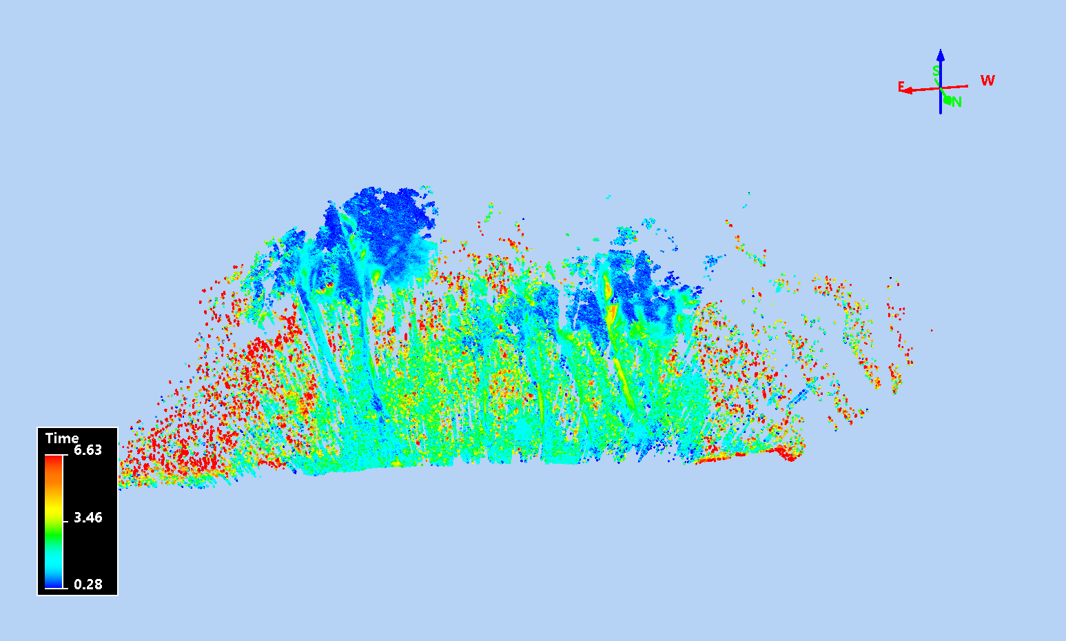
You'll see that our ground/snow classification wasn't perfect, and that a lot of trees stumps were left behind, leading to those red (high) HS values. Still, we get a good sense of snow distribution, and, if we do this process for a bunch of scans, we can analyse the change in HS over time.

Future work

It'd be nice to store the HS in a custom attribute, as well, so that software that can handle las extra bytes (e.g. CloudCompare) could display the data with correct labeling. But the current solution, in my opinion, is good enough!

Footnotes

Back to top