Slope maps with GMT
About two-thirds of dry slab avalanches occur on slopes between 30° and 45°. A map of slope angles is therefore a useful tool for safe decision making when backcountry skiing.
The excellent CalTopo provides a suite of map building tools, including a slope angle shading map. But me being me, I want to make my own maps.
This walkthrough describes how to make a slope angle shading map using free and open data and Generic Mapping Tools (GMT). You'll need the following softwares to follow along:
- GMT
- GDAL/OGR
The Makefile used in this example, along with a download script to fetch the map data, are in a gist at the bottom of this post.
The goal
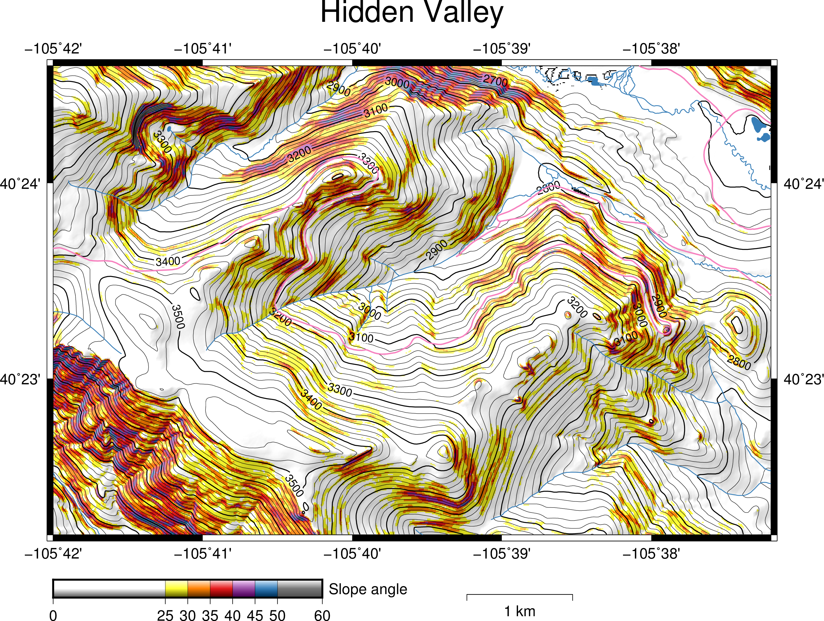
Hidden Valley is a abandoned ski area in Rocky Mountain National Park that closed in 1991. It now is a popular winter destination for backcountry skiing and sledding. We want to color-code dangerous slope angles while providing enough additional context to make a useful map.
Getting the data
We'll use data from the USGS 3D Elevation Program to produce our slope, hillshade, and contour grids. Our stream and lake overlays will come from the National Hydrography Dataset, and the roads from the National Transporation Dataset. All these products are browsable and downloadable through The National Map. All told, it's about 4.6G of data, organized like this on my system:
$ tree -P '*.shp|*.flt'
.
├── dem
│   ├── n40w106
│   │   └── n40w106.shp
│   ├── n41w106
│   │   └── n41w106.shp
│   ├── usgs_ned_13_n40w106_gridfloat.flt
│   └── usgs_ned_13_n41w106_gridfloat.flt
├── roads
│   └── Shape
│       ├── Trans_AirportPoint.shp
│       ├── Trans_AirportRunway.shp
│       ├── Trans_RailFeature.shp
│       ├── Trans_RoadSegment.shp
│       ├── Trans_RoadSegment2.shp
│       ├── Trans_RoadSegment3.shp
│       └── Trans_TrailSegment.shp
└── water
    └── Shape
        ├── NHDArea.shp
        ├── NHDFlowline.shp
        ├── NHDLine.shp
        ├── NHDPoint.shp
        ├── NHDPointEventFC.shp
        ├── NHDWaterbody.shp
        ├── WBDHU10.shp
        ├── WBDHU12.shp
        ├── WBDHU2.shp
        ├── WBDHU4.shp
        ├── WBDHU8.shp
        └── WBDLine.shp

7 directories, 23 files
Creating a simple raster map with GMT
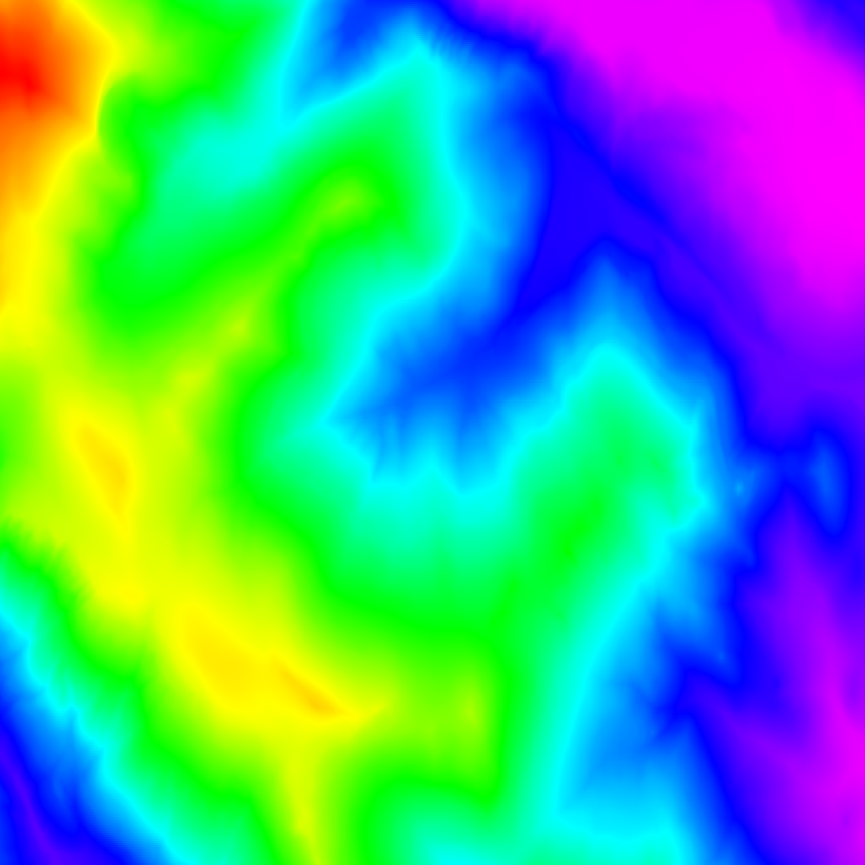
To prove that our system is working, let's create a rainbow elevation map from our DEM data in our area of interest.
We'll use a Makefile and place our generated products in build/.
First, we define our area of interest and create a rule for our build directory:
XMIN:=-105.70
XMAX:=-105.62
YMIN:=40.37
YMAX:=40.41

build:
 mkdir $@
Next, we subset our DEM data to our area of interest using a VRT. For some reason GMT (on my system) isn't happy reading VRTs, even though it should be able to use any GDAL-y data source, so we use the VRT to create a GeoTIFF:
build/dem.vrt: Makefile | build
 gdalbuildvrt -te $(XMIN) $(YMIN) $(XMAX) $(YMAX) $@ $(wildcard dem/*.flt)

build/dem.tif: build/dem.vrt
 gdal_translate $< $@
Finally, we create our simple rainbow elevation map.
I do this in two steps — first I create the PostScript file, then I use psconvert to turn it into a png:
build/hidden-valley.ps: build/dem.tif Makefile | build
 grdimage $< > $@

%.png: %.ps
 psconvert -TG -A -P $<
A few things to note:
grdimagetakes many more options, but for now we're keeping it simple.- The
psconvertcommand converts the PostScript file into a png with transparency (-TG), cropped (-A), and rotated into portrait mode (-P).
We make our map by running make build/hidden-valley.png:
Creating more derivative products
We've already created one derivative product, our cropped DEM build/dem.tif.
Let's create the rest of the products we need to make our map.
I'll step through the rules one-by-one and talk through what they're doing.
Calculate the slope
build/slope.nc: build/dem.tif
 grdgradient -fg $< -S$@ -D
 grdmath $@ ATAN PI DIV 180 MUL = $@
grdgradient does derivative math on gridded data.
In this case, we use the combination of the -D and -S options to write the magnitude of the gradient vector to a file, build/slope.nc.
We also need to specify -fg because our data is a geographic (lat/lon) grid and we need to convert those latitudes and longitudes to meters before calculating the gradient.
Once we've calculated the raw gradient magnitude, we convert that scalar value to an angle, in degrees, using grdmath.
Create a hillshade
build/gradient.nc: build/dem.tif
 grdgradient -fg $< -G$@ -A-45 -Nt0.6
In this case, we use grdgradient to create a hillshade.
We use -N to control the intensity of the hillshade — since we'll be drawing contours and additional overlays, we dial down the intensity to 0.6 so the map is a bit less noisy.
Crop and convert the vector data
OGR2GMT:=ogr2ogr -f GMT -spat $(XMIN) $(YMIN) $(XMAX) $(YMAX) -clipsrc spat_extent

build/flowline.gmt: water/Shape/NHDFlowline.shp
 $(OGR2GMT) $@ $<

build/waterbody.gmt: water/Shape/NHDWaterbody.shp
 $(OGR2GMT) $@ $<

build/roads.shp: $(wildcard roads/Shape/Trans_RoadSegment*.shp)
 ogr2ogr -f 'ESRI Shapefile' -spat $(XMIN) $(YMIN) $(XMAX) $(YMAX) -clipsrc spat_extent $@ $(word 1,$^)
 ogr2ogr -f 'ESRI Shapefile' -spat $(XMIN) $(YMIN) $(XMAX) $(YMAX) -clipsrc spat_extent -addfields $@ $(word 2,$^)
 ogr2ogr -f 'ESRI Shapefile' -spat $(XMIN) $(YMIN) $(XMAX) $(YMAX) -clipsrc spat_extent -addfields $@ $(word 3,$^)

build/roads.gmt: build/roads.shp
 ogr2ogr -f GMT $@ $<
Creating flowline (streams) and waterbody (lakes, etc) vectors is a simple matter of cropping the source data with ogr2ogr and writing it out in the GMT format.
Creating the roads file is a bit more tricky, since the road data comes in three seperate shapefiles.
I wasn't able to figure out how to -addfields to a GMT vector file, so I create an intermediate build/roads.shp, then convert that file to gmt.
Create a color palette
build/slope.cpt: Makefile
 makecpt -Cwhite,'#ffff33','#ff7f00','#e41a1c','#984ea3','#377eb8','#777777' -T0,25,30,35,40,45,50,90 -N > $@
This rule creates a color palette that we'll use for our slopes.
Putting it all together
Now that we've created all of the intermediate products, let's rewrite our PostScript rule to create our final map. I'll step through the rule components one-by-one, with an explanation immediately after.
build/hidden-valley.ps: build/dem.tif build/slope.nc build/gradient.nc build/flowline.gmt build/waterbody.gmt build/roads.gmt build/slope.cpt Makefile
Add all of our derivative products to ensure they get built.
grdimage build/slope.nc -Cbuild/slope.cpt -Ibuild/gradient.nc -Ba -B+t"Hidden Valley" -JM8i -Rbuild/slope.nc -K > $@
Draw the slope grid, colored with our custom palette.
The -JM8i specifies the projection for these data, in this case a Mercator projection that is 8 inches wide.
The -R instructs grdimage to use the bounds of the build/slope.nc grid as the bounds of the plot.
The -I option adds the hillshade, the -Ba adds a border, the -B+t titles the plot.
The -K option "keeps the output file open" so we can add more layers.
grdcontour build/dem.tif -C20 -A100 -J -R -K -O >> $@
Add contours spaced 20 meters apart, labelled every 100 meters.
The -J and -R options inherit the values used in the previous command, so we don't need to specify them again.
The -O option instructs grdcontour to output "overlay" PostScript that is meant to be appended onto PostScript data "kept open" with -K.
 psxy build/flowline.gmt -W0.6p,'#377eb8' -J -R -K -O >> $@
 psxy build/waterbody.gmt -G'#377eb8' -J -R -K -O >> $@
 psxy build/roads.gmt -W1p,'#f781bf' -J -R -K -O >> $@
Add the vector data.
The -W option specifies the pen used to draw lines, and the -G option specifies the fill.
psbasemap -Lx5.2i/-0.7i+c$(YMIN)+w1k -J -R -K -O >> $@
Add the length scale, set to 1km.
psscale -D0i/-0.7i+w3i/0.2i+h -Cbuild/slope.cpt -G0/60 -By+l"Slope angle" -I -O >> $@
Add the color legend.
Now you can run make build/hidden-valley.png and get your map!
Conclusion
By automating this map-generation, you can easily create maps for new areas. Here's the complete Makefile used for this example, along with a download script to grab the data you need: